10.3 Hydrocyclone Separator

The use of hydrocyclones is the standard method in the mineral processing industry of separating the particles in a slurry by size or by density. Hydrocyclones are continuously operating separating devices that utilize centrifugal forces to accelerate the settling rate of particles. They have achieved wide-spread use because of their simplicity, their durability, and their relatively low cost.

A typical hydrocyclone is shown in Figure 10.1. The lower portion of a hydrocyclone is a conical vessel with an opening at the bottom to allow for the removal of the coarse or heavier particles. The conical section is joined to a cylindrical section, the top of which is closed with the exception of an overflow pipe known as a vortex finder. The vortex finder prevents the feed material that enters the cylindrical section tangentially from going directly into the overflow. Separation occurs in the cylindrical section due to the existence of a complex velocity distribution that carries the coarse particles to the bottom and the fine particles out the top.

Figure 10.1  Hydrocyclones have become the standard separation device in a number of industries including both the mineral processing industry and the separations industry.

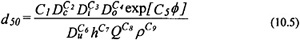
Plitt (1976) presented an empirical model to predict the d₅₀ or split size that is still used extensively today. The split size is that size particle (given by diameter of the particle) that has an equal chance of exiting the hydrocyclone either through the underflow or the overflow, and is often used to quantify the efficiency of this separation process. Plitt’s model has the following functional relationship:

where D_c, is the diameter of the hydrocyclone, D_i, is the diameter of the slurry input, D_o. is the diameter of the overflow, D_u is the diameter of the underflow, h is the height of the hydrocyclone, Q is the volumetric flow rate into the hydrocyclone, φ is the percent solids in the slurry input, and ρ is the density of the solids. The empirical constants, C_i, are selected so that the model accurately matches data that has been collected from actual hydrocyclone separators.

A number of approaches have been developed for determining the empirical constants associated with this particular model of a hydrocyclone. Most of the approaches involve the use of statistical routines, each of which has some potential drawbacks (Karr et al, 1995), many of which can be overcome by using a GA. The problem at hand is similar to the curve-fitting problem of Chapter 5. The coding scheme that was employed in the Ree-Eyring equation example of Chapter 5 is again used here. The fitness function of Chapter 5 is similar, except that the LS criteria has been replaced with the LMS criteria resulting in the following fitness function:

where f is the fitness function value, med is the median value, y is an actual data value, and y’ is an estimated data value using the parameters defined by a particular GA string.

A GA was used to select the values of C₁ through C₉ used in the empirical model of a hydrocyclone as shown in equation (10.1). Figure 10.2 demonstrates the effectiveness of using a GA for tuning the empirical constants. In this plot, the actual d₅₀ size is plotted against the d₅₀ size predicted using the model with the empirical constants as selected by a genetic algorithm. Note that the model would exactly reproduce the data if all of the points shown in Figure 10.2 fell on a line of 45°. Although the GA tuned model fits the data well for most of the data shown (excluding the outliers in the lower range of d₅₀) it systematically departs from the 45° line at high values of d₅₀. This modeling error indicates that either the GA has not determined the exact values of the coefficients or the mathematical relationship upon which the model is based is inadequate.

Figure 10.2  The GA tuned empirical model of the hydrocyclone separator matches the data obtained for real-world hydrocyclones well.

It is important to note that the GA determined the empirical constants in roughly 10 minutes, whereas a statistical package took roughly 9 hours to locate constants that provided the same quality fit to the data. This time of computation becomes critical when the tuning of an empirical model is being done as a part of a real-time, adaptive process control system such as the one discussed in Chapter 9.