The Finch and Doby model of column flotation consists of a number of empirical and semi-empirical equations that model individual aspects of flotation separately. Each of the equations has parameters that must be adjusted to fit conditions in a specific flotation cell. Many of these equations are concerned with calculating the number of collisions between the bubbles and the particles. These equations incorporate factors such as particle and bubble size and concentration, and the relative velocity between particles and bubbles. A very important equation is used to calculate the time it takes after collision for a particle to slide around the bubble. The net result of these various calculations is a rate constant for each species in the flotation cell. The Finch and Doby model of column flotation also relies heavily on a property of hydrophobic minerals called induction time. Induction time is the time required, once a hydrophobic particle has collided with a bubble, for the particle to attach to the bubble. If the induction time is less than the sliding time the bubble and particle become attached. Once the attachment has occurred, the particle will usually remain attached to the bubble until the bubble/particle aggregate rises to the liquid/froth interface level. Also, it is in practice often a good assumption that an ore particle that reaches the interface level will remain attached to its bubble and be carried out with the concentrate. The foam is sprayed with water to wash undesired and non hydrophobic particles back into the flotation cell.

Often the material concentrated by flotation will only be partially purified. If this is the case it must be re-floated in additional cells. In addition, some of the ore mineral will remain unfloated and this material must also be re-floated. The resulting assembly of flotation cells is called a flotation circuit. The exact amount of mineral removed by each flotation cell is determined by the residence time for a species in the flotation cell. The residence time is determined by a vessel dispersion number that is a measure of the degree of mixing in the vessel.

Data on the column circuit considered in this effort was presented in the thesis by Alford (1991). Alford’s data is taken from a circuit used in an industrial application at the Mount Isa Mines Limited installation in Australia

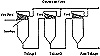
Figure 10.6  Column flotation units are used effectively in series as shown in the schematic above.

A GA has been used to tune selected parameters spread throughout a number of individual equations associated with flotation events in each column in order to make the values predicted by the model match as nearly as possible the behavior of the actual circuit as recorded by the data in Alford’s thesis. In addition it was necessary to determine a value for the vessel dispersion number. Since vessel dispersion number is largely a function of the size and shape of the column and since the physical dimensions of the three columns were identical, the three were assumed to have the same vessel dispersion number. Since induction time is a chemical property, the sphalerite and galena induction times were also assumed to be the same for each of the three columns.

The genetic algorithm was set up to minimize the mean squared error between the balanced data values based on observed flows in the Mount Isa Mines circuit and the corresponding values obtained from the computer model. There were 30 data values used in computing the mean squared error, and these data values included information about the percent solids, the percentage of lead, the percentage of zinc, the percentage of iron, and the flow volume in each of the six flows produced by the circuit. The final mean squared error attained by the genetic algorithm was 0.0003. The precise values achieved by the model are listed in Table 10.1 along with the balanced values based on observed data for comparison. (The percent solids column is omitted.) Each table entry is of the form V_m/V_b, where V_m is the value produced by the computer model and V_b is the balanced value from Alford’s data.