Initially, the selection of minimum and maximum values for each of the parameters seems to be an obvious decision; it seems that the minimum and maximum parameter values should simply coincide with the lower and upper limits of a variable’s range, i.e., the minimum value of the parameters for the membership functions describing E is -25 and the maximum value is 25. However, the selection of minimum and maximum values for each of the membership functions is at present subject to three constraints. The first constraint requires that each parameter value fall in the range selected by the user to represent each variable. The second constraint is that the definition of the linguistic terms should be consistent with the normal meaning of the terms. For example, the membership function associated with the term NEGATIVE BIG should be zero for positive numbers and near-zero for small negative numbers. The third constraint is that each point in the range being described should have at least one membership value assigned to it. In Figure 6.3 all the points on the E-axis have membership values defined by one or more of the membership functions except for those between -15.0 and -10.0. This is not acceptable. Membership functions must be constructed so that all relevant points have a membership value. Figure 6.4 illustrates a method for assuring that all points are associated with appropriate membership function values. Here, each point is allowed to slide within a pre-defined window bounded by values of C_min and C_max. The permitted ranges are selected by the user, but, as shown in the figure, these ranges must assure that there will be a small degree of overlap of the membership functions.

Actually, the three constraints listed above should be viewed as soft constraints. Generally speaking, they are solid guidelines the user should follow. However, there are situations in which these constraints can be violated, yet viable fuzzy systems can still be obtained. Later in this book, we will encounter such situations. For example, the hexamine controller we introduce in Chapter 15 employs a GA to continuously adjust membership functions in real-time. The hexamine controller will actually have gaps in portions of the state space in which the controller is not currently operating. However, since adjustments are being made continuously, the gaps are eliminated before the controller operates in that region of state space. For now, the three constraints will be followed for two reasons: (1) they are intuitive and (2) they will help keep us out of trouble.

Figure 6.3  If the values of C_min and C_max are not selected carefully, controllers with gaps in their condition variable ranges can result. These gaps are indicated by regions for which the fuzzy sets do not overlap.

Figure 6.4  The values of C_min and C_max shown above eliminated the possibility of a GA considering fuzzy systems with gaps in them.

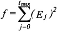
6.2.2 Fitness Function

The fitness function employed by a GA used to locate efficient fuzzy membership functions is directly tied to the goal of the control system. In a liquid level controller, the goal is to drive the liquid level to and maintain the level at a given setpoint in a minimum amount of time; that is to drive E and ΔE to zero in the shortest time possible. Thus, the fitness function must in some way include a concept of time.

Early in the research project, in discussing potential fitness functions for membership function selection in the liquid level problem, we considered numerous methods. For example, we discussed the ideas of minimizing energy consumption, of ensuring a critically damped system, and of never allowing the system to move further from the desired state. However, these discussions always seemed to return to plots of the liquid level versus time like that shown in Figure 6.5. In this figure, the vertical lines depict an error, E, at any particular time. The objective is not to have a controller that minimizes any individual error term, rather it is to minimize the sum of these error terms. Thus, the choice of fitness function for the liquid level problem must capture this idea:

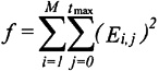
where f is the fitness function value, E is the error (difference between the current value of h and the setpoint defined for h), and t_max is the maximum time for which the computer simulation of the liquid level system is to be run. This definition of fitness function allows the GA to discover membership functions for effective control of the liquid level system from a given initial condition. However, the goal was to control the liquid level system beginning from any initial condition.

Thus, the fitness function described in Equation 6.2 above was extended to capture the idea that any initial condition could be considered. The second iteration of the fitness function used for the liquid level controller was:

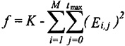
where M is the number of initial condition cases considered. Unfortunately, since the liquid level system can be in any of an infinite number of initial states, every initial condition cannot be considered. However, when the initial condition cases are selected carefully to represent the extreme regions of state space (maximum and minimum values of E and ΔE), an efficient and robust controller can be developed.

The only apparent problem associated with the fitness function of Equation (6.3) is that it is a value that we seek to minimize. As you recall, the GA described in Chapter 5 seeks to maximize fitness. Thus, the fitness function actually used in this effort (and used in the design of many controllers introduced later in this book) is:

where K is a large constant selected to ensure that the value of f remains positive. By employing the fitness function of Equation 6.4 above, a GA was able to design a liquid level controller that was more efficient than the controller presented in Chapter 2.