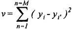
5.2.3 Fitness Function

Now that each string has some “meaning” in our particular curve-fitting problem, the GA requires us to provide a value of relative merit for each possible solution; a fitness function that informs the GA of how close it is to achieving our objective. In this problem, our objective is to minimize the sum of the residuals between the data points and our particular curve. Mathematically, we want to minimize the following

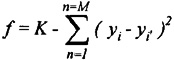
where v is the value to be minimized, y_i is the value of f(x) associated with data point i, y_I’ is the corresponding value of f(x) predicted by the model equation, y_I’ = mx_i + b, and M is the number of data points.

This value v, however, does not correspond directly to the fitness value needed by a GA. Although GA operators have been developed that can be used for minimization problems, the operators used in this chapter (to be introduced shortly) allow only for solving maximization problems. Thus, we must convert our minimization problem into a maximization problem. To do this, we will simply subtract the value of v from a large number. Thus, an acceptable fitness value, f, is as follows

where K is a constant just large enough to make all of the fitness values greater than zero. In the current example, K = 25.0. This function requires good solutions to have fitness values that are larger than those of poor solutions. With this in mind, Table 5.5 shows the fitness values associated with each of the strings in the initial generation.

5.2.4 Generate New Solutions

At this point, we have obtained five random possible solutions to the least-squares problem. It is time to work some GA magic through which the information contained in this initial generation will produce subsequent generations that contain better solutions to the problem.

The next step in the process is to apply the GA operators. Although numerous high-powered, problem-specific GA operators have been developed and used successfully, most problems can be solved very effectively using only three basic operators: (1) reproduction, (2) crossover, and (3) mutation.

The first operation, reproduction, allows strings with large fitness values, good solutions to the problem at hand, to receive many copies in the new population. In this chapter, use is made of a particular type of selective reproduction, called expected number control. This form of selective reproduction makes a certain number of copies, numi, of a string in accordance with the equation:

Thus, reproduction is the survival-of-the-fittest aspect of the GA. The best strings receive more copies in subsequent generations so that their desirable traits can be passed to their offspring. It should be apparent that in this form of reproduction, high quality strings must have large values of fitness because the GA is going to maximize the fitness values.

The newly formed strings are placed in a file, generally called a mating pool, where they await application of the second and third operators. Table 5.6 depicts the mating pool resulting from the application of the reproduction operator to the initial generation. Notice that the mating pool does not contain any strings that were not represented in the initial generation, only copies of the selected strings. Rather, the reproduction process has simply exploited the fitness function to bias the new population toward high-quality strings. Thus, the remaining operators must produce strings containing new and better parameter values if we ever hope to get significantly better solutions than those represented by the initial, randomly generated population. The remaining operators must generate parameter values that have not yet been considered; they must investigate new points in the search space.