|
|
|
|||
        |
|
|
|
[an error occurred while processing this directive]
THEOREM 12.6 Suppose that algorithm A determines quadratic residuosity correctly with probability at least 1/2 + ε. Then the algorithm A1, as described in Figure 12.8, is a Monte Carlo algorithm for Quadratic Residues with error probability at most 1/2 + ε. PROOF For any given input The last step is to show that any (unbiased) Monte Carlo algorithm that has error probability at most 1/2 + ε can be used to construct an unbiased Monte Carlo algorithm with error probability at most δ, for any δ > 0. In other words, we can make the probability of correctness arbitrarily close to 1. The idea is to run the given Monte Carlo algorithm 2m + 1 times, for some integer m, and take the “majority vote” as the answer. By computing the error probability of this algorithm, we can also see how m depends on δ. This dependence is stated in the following theorem.
THEOREM 12.7 Suppose A1 is an unbiased Monte Carlo algorithm with error probability at most 1/2 + ε. Suppose we run A1 n = 2m + 1 times on a given instance I, and we take the most frequent answer. Then the error probability of the resulting algorithm is at most
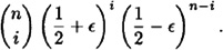
PROOF The probability of obtaining exactly i correct answers in the n trials is at most
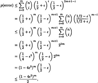
The probability that the most frequent answer is incorrect is equal to the probability that the number of correct answers in the n trials is at most m. Hence, we compute as follows
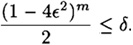
as required. Suppose we want to lower the probability of error to some value δ, where 0 < δ < 1/2 - ε. We need to choose m so that
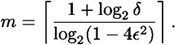
Hence, it suffices to take
Then, if algorithm A is run 2m + 1 times, the majority vote yields the correct answer with probability at least 1 - δ. It is not hard to show that this value of m is at most c/(δε2) for some constant c. Hence, the number of times that the algorithm must be run is polynomial in 1/δ and 1/ε. Example 12.5 Suppose we start with a Monte Carlo algorithm that returns the correct answer with probability at least .55, so ε = .05. If we desire a Monte Carlo algorithm in which the probability of error is at most .05, then it suffices to take m = 230 and n = 461. Let us combine all the reductions we have done. We have the following sequence of implications: Since it is widely believed that there is no polynomial-time Monte Carlo algorithm for Quadratic Residues with small error probability, we have some evidence that the BBS Generator is secure. We close this section by mentioning a way of improving the efficiency of the BBS Generator. The sequence of pseudo-random bits is constructed by taking the least significant bit of each si, where 12.4 Probabilistic EncryptionProbabilistic encryption is an idea of Goldwasser and Micali. One motivation is as follows. Suppose we have a public-key cryptosystem, and we wish to encrypt a single bit, i.e., x = 0 or 1. Since anyone can compute eK (0) and eK (1), it is a simple matter for an opponent to determine if a ciphertext y is an encryption of 0 or an encryption of 1. More generally, an opponent can always determine if the plaintext has a specified value by encrypting a hypothesized plaintext, hoping to match a given ciphertext. The goal of probabilistic encryption is that “no information” about the plaintext should be computable from the ciphertext (in polynomial time). This objective can be realized by a public-key cryptosystem in which encryption is probabilistic rather than deterministic. Since there are “many” possible encryptions of each plaintext, it is not feasible to test whether a given ciphertext is an encryption of a particular plaintext. Here is a formal mathematical definition of this concept. DEFINITION 12.3 A probabilistic public-key cryptosystem is defined to be a six-tuple
Copyright © CRC Press LLC
|
 |
         |
|
 , the effect of step 2 in algorithm A1 is to produce an element x′ that is a random element of
  whose status as a quadratic residue is known.
)

)
 mod n. Suppose instead that we extract the m least significant bits from each si. This will improve the efficiency of the PRBG by a factor of m, but we need to ask if the PRBG will remain secure. It has been shown that this approach will remain secure provided that m ≤ log2 log2 n. So we can extract about log2 log2 n pseudo-random bits per modular squaring. In a realistic implementation of the BBS Generator,
  , so we can extract nine bits per squaring.
 where
where  is the set of plaintexts,
  is the set of ciphertexts,
  is the keyspace,
  is a set of randomizers, and for each key
  ,
,  is a public encryption rule and
  is a secret decryption role. The following properties should be satisfied:
 and
and  are functions such that
 and every
  . (In particular, this implies that
  .)
.)
 and for any
  , define a probability distribution pK,x on
  , where pK,x(y) denotes the probability that y is the ciphertext given that K is the key and x is the plaintext (this probability is computed over all
  ). Suppose
  , x ≠ x′, and
  . Then the probability distributions pK,x and pK,x′ are not ε-distinguishable.