|
|
|
|||
        |
|
|
|
[an error occurred while processing this directive]
Example 4.7 Consider the Jacobi symbol
Suppose n > 1 is odd. If n is prime then
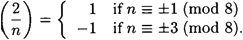
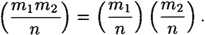
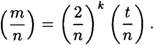
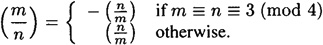
However, it can be shown that, for any odd composite n, n is an Euler pseudo-prime to the base a for at most half of the integers a such that 1 ≤ a ≤ n - 1 (see the exercises). This fact shows that the Solovay-Strassen primality test, which we present in Figure 4.7, is a yes-biased Monte Carlo algorithm with error probability at most 1/2. At this point it is not clear that the algorithm is a polynomial-time algorithm. We already know how to evaluate a(n-1)/2 mod n in time O((log n)3), but how do we compute Jacobi symbols efficiently? It might appear to be necessary to first factor n, since the Jacobi symbol Fortunately, we can evaluate a Jacobi symbol without factoring n by using some results from number theory, the most important of which is a generalization of the law of quadratic reciprocity (property 4 below). We now enumerate these properties without proof:
Example 4.8 As an illustration of the application of these properties, we evaluate the Jacobi symbol
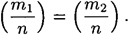
Notice that we successively apply properties 4, 1, 3, and 2 in this computation. In general, by applying these four properties, it is possible to compute a Jacobi symbol Suppose that we have generated a random number n and tested it for primality using the Solovay-Strassen algorithm. If we have run the algorithm m times, what is our confidence that n is prime? It is tempting to conclude that the probability that such an integer n is prime is 1 - 2-m. This conclusion is often stated in both textbooks and technical articles, but it cannot be inferred from the given data. We need to be careful about our use of probabilities. We will define the following random variables: a denotes the event
and b denotes the event
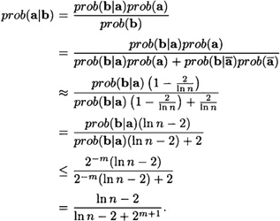
It is certainly the case that prob(b|a) ≤ 2-m. However, the probability that we are really interested is prob(a|b), which is usually not the same as prob(b|a). We can compute prob(a|b) using Bayes’ theorem (Theorem 2.1). In order to do this, we need to know prob(a). Suppose N ≤ n ≤ 2N. Applying the Prime number theorem, the number of (odd) primes between N and 2N is approximately
Since there are
Then we can compute as follows:
Note that in this computation,
It is interesting to compare the two quantities (ln n - 2)/(ln n - 2 + 2m+1) and 2-m as a function of m. Suppose that Although 175/(175+2m+1) approaches zero exponentially quickly, it does not do so as quickly as 2-m. In practice, however, one would take m to be something like 50 or 100, which will reduce the probability of error to a very small quantity. We conclude this section with another Monte Carlo algorithm for Composites which is known as the Miller-Rabin algorithm (it is also known as the “strong pseudo-prime test”). This algorithm is presented in Figure 4.9. It is clearly a polynomial-time algorithm: an elementary analysis shows that its complexity is O((log n)3), as in the case of the Solovay-Strassen test. In fact, the Miller-Rabin algorithm performs better in practice than the Solovay-Strassen algorithm. We show now that this algorithm cannot answer “n is composite” if n is prime, i.e., the algorithm is yes-biased.
Copyright © CRC Press LLC
|
 |
         |
|
 . The prime power factorization of 9975 is 9975 = 3 × 52 × 7 × 19. Thus we have
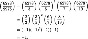
 (mod n) for any a. On the other hand, if n is composite, it may or may not be the case that
  (mod n). If this equation holds, then n is called an Euler pseudo-prime to the base a. For example, 91 is an Euler pseudo-prime to the base 10, since
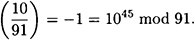
 is defined in terms of the factorization of n. But, if we could factor n, we would already know if it is prime, so this approach ends up in a vicious circle.
)
 as follows:
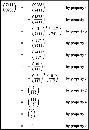
 in polynomial time. The only arithmetic operations that are required are modular reductions and factoring out powers of two. Note that if an integer is represented in binary notation, then factoring out powers of two amounts to determining the number of trailing zeroes. So, the complexity of the algorithm is determined by the number of modular reductions that must be done. It is not difficult to show that at most O(log n) modular reductions are performed, each of which can be done in time O((log n)2). This shows that the complexity is O((log n)3), which is polynomial in log n. (In fact, the complexity can be shown to be O((log n)2) by more precise analysis.)
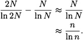
 odd integers between N and 2N, we will use the estimate
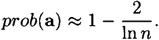
 denotes the event
)
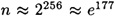 , since these are the sizes of primes that we seek for use in RSA. Then the first function is roughly 175/(175 + 2m+1). We tabulate the two functions for some values of m in Figure 4.8.